10. Area and Average Value

d. Average Value and Mean Value Theorem

Recall: The average value of a function \(f(x)\) on an interval \([a,b]\) is: \[ f_\text{ave}=\dfrac{1}{b-a}\int_a^b f(x)\,dx \]

3. Mean Value Theorem for Integrals

Next notice that the average value of a function \(f\) on an interval \([a,b]\) is always between the minimum and maximum values of \(f\) on the interval \([a,b]\).

If \(m\) is the minimum and \(M\) is the maximum, then: \[ m \le f(x) \le M \] \[ \int_a^b m\,dx \le \int_a^b f(x)\,dx \le \int_a^b M\,dx \] \[ m(b-a) \le \int_a^b f(x)\,dx \le M(b-a) \] \[ m \le f_\text{ave} \le M \]

Consequently, by the Intermediate Value Theorem, if \(f(x)\) is continuous on \([a,b]\), then there is a number \(c\) in \([a,b]\) where \(f(c)=f_\text{ave}\). Thus we conclude:

If \(f(x)\) is a continuous function on the interval \([a,b]\), then there is a number \(c\) in \([a,b]\), where: \[ f(c)=f_\text{ave}=\dfrac{1}{b-a}\int_a^b f(x)\,dx \]

The number \(c\) may or may not be unique.

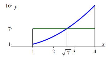
Find the number(s) \(c\) guaranteed by the Mean Value Theorem for Integrals for the function \(f(x)=x^2\) on the interval \([1,4]\).

The average value was found in a previous example to be \(f_\text{ave}=7\). So we need to solve \(f(c)=f_\text{ave}\) or \(c^2=7\). Therefore \(c=\sqrt{7}\). This is the point where the green line crosses the blue curve in the graph:

Notice the solution \(c=-\sqrt{7}\) is not in the interval \([1,4]\).

Your turn:

Find the number(s) \(c\) guaranteed by the Mean Value Theorem for Integrals for the function \(f(x)=(x-2)^2\) on the interval \([1,3]\).

\(c=2\pm\dfrac{1}{\sqrt{3}}\)

The average value was found, in a previous exercise, to be \(f_\text{ave}=\dfrac{1}{3}\). So we need to solve \((c-2)^2=\dfrac{1}{3}\). Therefore \(c_\pm=2\pm\dfrac{1}{\sqrt{3}}\). These are the two points where the green line crosses the blue curve in the graph:

10. Area and Average Value

d. Average Value and Mean Value Theorem

3. Mean Value Theorem for Integrals

Heading